|
PMF Modeling
|
| Introduction |
| |
|
In order to identify the sources of aerosols in the Fish
and Wildlife Class I Areas in the central and eastern United States,
Positive Matrix Factorization (PMF) receptor model is applied to the 24-hr
integrated aerosol chemical composition data obtained through the
Interagency Monitoring of Protected Visual Environments (IMPROVE) program.
PMF is applied to each site to generate profiles of source factors.
Normalized source profiles and the quantitative source contributions for
each resolved factor are calculated. |
| |
| Model Description |
| |
|
PMF is a statistical method that identifies a user
specified number of source profiles (i.e. relative composition particle
species for each source) and source strengths for each sample period that
reduce the difference between measured and PMF fitted mass concentration.
Equations 1 – 4 show the major steps of the model calculation. |
| |
 (1)
(1) |
| |
where: X (n * Sp) = a matrix of observed
fine particulate species concentrations with the dimensions of number of
observations by the number of species
G (n * f) = a matrix of source contributions by observation day with the
dimensions of number of observations by the number of factors
F (f * Sp) = a matrix of source profiles with the dimensions of number of
factors by the number of species
E (n * Sp) = a matrix of random errors with the dimensions of number of
observations by number of species |
| |
The F and G matrices of the final
solution are then normalized according to the following equations to
determine the quantitative source contributions (Ci, µg/m3)) and profiles
for each source (Si, µg/µg).
|
 (2)
(2) |
where: Si = the row of the source profile
matrix for source i
Fij = the source profile value for specie j of source i
FMi = the calculated average total fine mass contribution for source i |
| |
 (3)
(3) |
where: Ci = the column of the source
contribution matrix for source i
Gki = the source contribution on day k for source i
FMi = the calculated average total fine mass contribution for source i
|
|
The FMi is
determined by regression total PM2.5 mass concentrations in the
kth sample (mk) against estimated source
contribution values. |
 (4)
(4) |
| |
| Input Data |
| |
|
1. Download aerosol PM10 and PM2.5 mass and chemical
speciation data including analytical uncertainty and minimum detection limit
from the VIEWS web site. |
| |
|
2. Data are screened to remove the days when PM10 or
PM2.5 mass concentration or concentration of any major aerosol component is
missing.
Table 1 lists all the concentrations measured by IMPROVE and the fraction of
the measurement values that are below the minimum detection limit based on
all the data available from all the sites. The components with measurement
values below the detection limit more than 50% of the time, except major
components including EC3, OC1, Chloride and Sodium as marked gray, are not
included in the PMF modeling and marked red in the table. As sulfate and
sulfur are highly correlated (slope = 3, R2 = 0.96), only sulfur is included
in the PMF modeling. Therefore, a total of 29 species are included in the
PMF modeling. |
| |
| 3. Data value and associated uncertainty
are calculated as: |
| |
If data is missing Then
data value = geometric mean of the measured values
uncertainty = 4 * geometric mean of the measured values
Else if data bellows detection limit
data value = 1/2 * detection limit
uncertainty = 5/6 * detection limit
Else
data value = measured data
uncertainty = analytical uncertainty + 1/3 * detection limit
|
| |
| Table 1. Fraction of the measurement
values that are below the minimum detection limit. Red:>50% below detection
limit, not included in PMF, Gray: >50% below detection limit, still included
in PMF and Yellow: not included in PMF |
 |
| |
| |
| Major Control Parameters |
| |
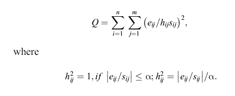
| 1. Running Mode: Robust Mode, the
value of outlier threshold distance a = 4.0 (i.e. if the residue exceeds 4
times of the standard deviation, a measured value is considered outlier).
The least squares formulation thus becomes: |
 |
| |
2. Error Mode (decides the
standard deviation of the data Sij):
EM = -12 (based on observed value) Sij = Tij |
| |
| 3. FPEAK and FKEY Matrix (controls
the rotation) – default: 0 (central), may try different numbers |
| |
| Determination of the number of sources
(factors) |
| |
| Then the following methods are used to
decide how many factors (sources) should be chosen for each area. |
| |
| 1. The regression coefficients FMi should
be positive. If the regression produces a negative coefficient, it suggests
that maybe too many source factors have been used. |
| |
| 2. The sum of the scaled profiles should
be less than unity. If any of them is much higher than unity (i.e. >2) it
suggests that too few sources may have been chosen. |
| |
| 3. Other PMF output parameters: |
| |
| a. Q value |
| |
b.
 |
c.
 |
| d. Largest element in Rotmat matrix |
| |
| 4. Judgement based on literature, known
CMB source profiles, and experience |
| |
| Output Data |
| |
| 1. Source (factor) profiles for each
site. |
| |
| Source (factor) profiles (see example as
shown in Figure 2) which represent the fraction of each aerosol component to
total PM2.5 mass for PMF defined sources (factors) are calculated for each
site. |
| |
 |
| Figure 2. Example source (factor) profile
(unit: mg/mg) based on PMF modeling |
| |
| 2. Contribution of each source (factor)
to aerosol mass and light extinction for each sampling day. |
| |
| For each IMPROVE site in the Fish and
Wildlife Class I Areas in the eastern and central US, contributions of each
source (factor) to aerosol mass and light extinction for each sampling day
are calculated (see example as shown in Figure 3). |
| |
 |
| Figure 3. Contributions of major aerosol
sources to PM2.5 mass during the sampling days of 2004 (example). |
| |
| Naming Factors |
| |
|
Generally, source factors are identified based on the PMF generated source
profiles (signatures). The biomass smoke factor is dominated by OC/EC with
significant amount of K, while secondary sulfate and nitrate factors are
dominated by sulfate and nitrate, respectively. Major dust components such
as silicon, calcium, iron, and potassium are present in the dust factor.
Vanadium and Nickel, which are almost exclusively from oil combustion, are
used as the signatures of the oil combustion source factor (e.g. shipping
emissions). A mobile emission factor is identified with large fraction of OC/EC,
and metals such as Zn, Pb and Cd. Generally, EC dominates in diesel
emissions and OC dominates in gasoline emissions. Se, As and Sb are tracers
for coal combustion sources. Of course, large amount of OC/EC and sulfate
always exit in coal combustion emissions. Sodium and chlorine (or chloride)
are the major aerosol species in sea salt aerosols. Emissions from Kraft
recovery boilers of paper mills have been shown to consist largely of sodium
and sulfate particles (i.e. Na2SO4) with lesser but
significant amounts of Chlorine and Potassium. |
| |
| |