| 3.2 Methodology |
|
| We used the same air mass
trajectories from the section 5 to determine representative sites near to
each tribe. For this analysis we considered point source emissions obtained
from the EPA National Emision Inventory (NEI) for 2002. Of the NEI we
include sources of NOx and SO2 only. The effects of urban areas were
considered indirectly since high densities of NOx sources tend to correlate
with urbanized areas and less for the outlying rural areas. |
|
| In a similar fashion to task
2, we calculated buffer zones around each tribal centroid. To account for
the fact that smaller emission sources contribute to ambient concentrations
much less than larger sources, we devised a simple method to generate
emission source buffer zones around each point source. These emission source
buffer zones act as radius of impact for each source. Instead of running a
source model for each point, we generalized the source according to its
annual emission rate in tons per year. The radius of impact of various
classes of point sources was then calculated using the EPA SCREEN3
dispersion model. The SCREEN3 model predicts the worst case ambient air
impacts from a single source assuming poor dispersion conditions. We used
the SCREEN3 model as packaged through the Screen View freeware software
distributed by Lakes Environmnetal. Stack inputs for the model were chosen
based on a sampling of typical sources and source emission rates from the
National Emission Inventory. For those emissions given in tons per year (TPY),
we assumed a 24-hour operation to calculated an hourly emission rate in
pounds per hour. |
|
|
| Emission Rate (TPY) |
Emiss.Rate (lb/hr) |
Stack Height (ft) |
Stack Dia (ft) |
Stack Vel (m/s) |
Stack Exit Temp (F) |
Ambient Temp (F) |
| 50 |
11.4 |
50 |
3 |
30 |
200 |
67.7 |
| 500 |
114.2 |
100 |
5 |
30 |
200 |
67.7 |
| 2000 |
456.6 |
483 |
18.2 |
18.3 |
158 |
67.7 |
| 10000 |
2283.1 |
483 |
18.2 |
18.3 |
158 |
67.7 |
| 77860 |
17776.3 |
483 |
18.2 |
18.3 |
158 |
67.7 |
|
|
| The SCREEN3 model was run for
each emission rate category and a radius of influence matrix was assembled
for three averaging times of 3-hr, 24-hr and annual averages. The three
averaging times were chosen based on the averaging times of the National
Ambient Air Quality Standards as well as for New Source Review Prevention of
Significant Deterioration increment analysis. We used significance levels of
1 µg/m3 for annual averages, 5 µg/m3 for 24-hour averages and 25 µg/m3 for
3-hour averages. The radius of influence was determined based on the
distance the SCREEN3 based single-source concentration tailed-off to the
concentration of the significance level. The results of this analysis are
shown in Table 6-2 for the five different source categories. The model based
radius of influence were used to make continous categories of radius of
influence as shown in Table 5-2 in the column labeled Adjusted Radius. While
some of the model based radius of influence values were over the Adjusted
Radius, the overall trend toward larger radii for larger emissions was
preserved. |
|
| NOX, SO2 (TPY) |
Radius of Influence (km) |
Adjusted Radius (km) |
NOx, SO2 range in GIS |
| 3-hr |
24-hr |
Annual |
| 50 |
0.3 |
0.5>50 |
6 |
5 |
0 - 50 |
| 500 |
40 |
10 |
>50 |
20 |
50 - 500 |
| 2,000 |
0.7 |
>50 |
20 |
40 |
500 - 2,000 |
| 10,000 |
>50 |
>50 |
>50 |
60 |
2000 - 10,000 |
| 77,860 |
>50 |
>50 |
>50 |
80 |
10,000 - 77,860 |
| Significance Level (µg/m3) |
25 |
5 |
1 |
|
|
|
|
| After the radius of influence
was calculated for each source, it was incorporated into computer program
that processed the trajectories along with the tribal buffer zones. For
every forward and backward trajectory, the emissions were summed up as the
air parcel traveled from the IMPROVE site to the tribe. The emission point
was included in the sum only if the trajectory intersected the radius of
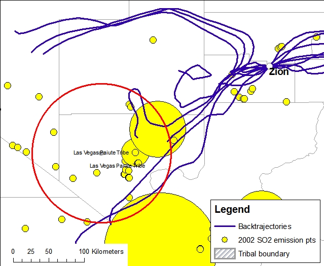
influence. This is illustrated in Figure 5-1 while considering ZION1 as a
potential representative site for the Las Vegas Paiute Tribe. Here we only
present 24-hours worth of trajectories from the ZION1 site. |
|
 |
|
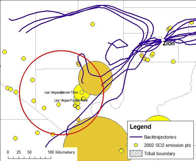
| In this example only those
trajectories that eventually intersect the Las Vegas Paiute Tribe’s buffer
zone are considered in the calculation. For those trajectories that
intersect the tribe’s buffer zone, we then determine which emission points
the trajectory intersects and sum up the emissions in tons per year. The
emission points that were included in the sum are shown in Figure 5-2 as
colored in with dark yellow. |
|
 |
|
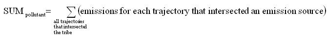
| Similar to task 2, we devised
a useful representativeness metric that considered total emissions between
the tribe and the nearby IMPROVE sites as well as taking into consideration
the distance. We define sites with lower metric scores a better choice for
being representative than those with higher scores. The sum of emissions
over all trajectories was weighted by the distance, R, in kilometers from
the tribe to the IMPROVE site. The weighting of R2 provides a way to weight
the closer sites more than the distant sites. |
|
 |
|
|
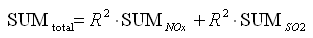
| Since we considered the two
pollutants, NOx and SO2, the metric becomes, |
|
 |
|
|
| The SUMtotal metric was
calculated for each tribe/IMPROVE site pair. We then eliminated the furthest
sites, those IMPROVE sites more than 400 kilometers from the tribe. The
closest site was selected as well as the sites that were within 20 percent
of that distance. Of those sites, we ranked them according to the SUMtotal
metric. The selected site chosen as the most representative was the one with
the lowest SUMtotal value. |
|
|
|
|